The logistic map was popularized in a now-canonical work by biologist Robert May (1976). It is important because it shows how both linear and nonlinear patterns can emerge from a simple equation for population growth \[ P_{t+1} = {r P_t(1-P_t)}\]
The population in the next generation Pt+1 is determined by the population in the current generation Pt, the rate at which individuals reproduce r, and the level of available resources given that the system has a finite carrying capacity, 1 – Pt.
The equation is interesting because it is extremely simple while displaying remarkably rich behavior. For small values of r, the equation is deterministic: the increase in P is proportional to the increase in r. However, at a key point, the population begins to oscillate between two values, then later at four values, then at 8 values, 16, 32, etc. Regular oscillations are quickly replaced by chaotic fluctuations (r ≳ 3.569); at these growth rates, tiny differences in the initial population yield all possible final population sizes within a given range. Even more astonishingly, in places, islands of stability appear (the white 'gaps' in the figure below).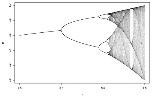
Thus merely varying the growth rate in the simplest possible equation for population growth generates linear, oscillatory or chaotic behavior. In the language of complexity science, or more specifically of nonlinear dynamics, each of these states is called a regime, or attractor. As long as the growth rate is less than a certain value, the behavior is linear. But if the growth rate happens to fall within the chaotic regime, prediction is practically impossible; the slightest error in parameter estimation cascades over time, and observed and anticipated P will diverge.
Explore these behaviors by changing the starting population P0 and growth rate r in the app below. (If the plots are not visible, click the '↺ Reset' button). The lower graph shows 30 time steps of the logistic equation, given the initial conditions P0 and r that you choose. To emphasize the sensitivity of the equation to initial conditions, results are also shown for P0 – 0.05 and P0 + 0.05. The behavior observed over longer time frames (here, 70 to 120 time steps) is shown in the bifurcation diagram above the time series.
Questions:- What kinds of relationships can you see between the population time series graph (lower) and the bifurcation diagram (upper)?
- Can you identify regions where the behavior is linear, chaotic or stable?
- At approximately which values of r do these transitions occur?
Note that the behavior observed over longer time frames (here, 70 to 120 time steps) is shown in the bifurcation diagram above the time series when the 'Static, skip t<50' box is ticked (default). You can instead use the 'Responsive' option to get a better impression of the approach of P to stable points (or to the chaotic region) depending on P0 and r. Here, time steps 0 to 70 are plotted, with initial condition P0.
References:
May RM. 1976. Simple mathematical models with very complicated dynamics. Nature 261:459-67.
May RM. 1976. Simple mathematical models with very complicated dynamics. Nature 261:459-67.